Tip: Are you a non-native English speaker? I have just finished creating a
  Web App
People often tend to learn inequalities just as formulas that are to be memorized, not to be thought about. There is, however, usually an intuitive explanation of the inequality which allows you the understand what it actually means. In this article, I’ll try to provide such an explanation for the Cauchy-Schwarz inequality, Markov’s inequality, and Jensen’s inequality.
Cauchy-Schwarz inequality
Let $x, y ∈ V$ where $V$ is any inner-product space, i.e. it is equipped with an inner product $⟨⋅, ⋅⟩: V × V → ℝ$. The Cauchy-Schwarz inequality says that $$|⟨x,y⟩| ≤ ‖x‖‖y‖\,,$$ where $‖x‖ = √{⟨x,x⟩}$ is the norm (the length) of $x$. To be able to understand the inequality, it is essential to understand what an inner product means. Let $u ∈ V$ be a unit vector, i.e. a vector with $‖u‖ = 1$ (you can imagine the vector $(1,0) ∈ ℝ^2$, for example). For any $v ∈ V$, $⟨u,v⟩$ is the length of the projection of $v$ to the direction $u$.
By dividing both sides of the Cauchy-Schwarz inequality by $‖x‖‖y‖$ and using the fact that constants can be put inside any inner product, we can rewrite the inequality as
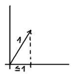 If you divide a vector by its length, the resulting vector has length $1$, i.e. it is a unit vector, so the inequality says just the following: The length of the projection of a unit vector ($y/‖y‖$) to some direction ($x/‖x‖$) is less than or equal to $1$. In other words, if you project a vector, it cannot get longer (look at the image on the right). The inequality is often used in the context of $L^2(μ)$ spaces where $μ$ is a measure. Then a scalar product is defined as $⟨f,g⟩ = ∫ fg\,dμ$, and the inequality holds for any two $f,g ∈ L^2(μ)$, and although these spaces are usually infinite-dimensional, I consider the geometric intuition mentioned above still appropriate in this case.
Markov’s inequality
Markov’s inequality can most naturally be stated in the language of probability theory—let $\P$ be a probability measure, $X$ a non-negative random variable, and $\E$ the expectation with respect to $\P$ (i.e. $\E[X] = ∫X\,d\P$, the weighted average of $X$). Then $$\P(X≥a) ≤ ÷{\E[X]}{a}$$ for all $a > 0$. But there is also another way to write this—by choosing $a = c\E[x]$. Then $$\P(X≥c\E[X]) ≤ ÷{1}{c}\,.$$ That means that the probability that $X$ is $c$ times larger than it’s average is at most $÷{1}{c}$. But of course it is; if it were more, say $p > ÷{1}{c}$, the expectation (i.e. the average) would be at least $c\E[X]⋅p > \E[X]$. For example, if $\P(X ≥ 3) = 0.5$, then it’s not possible that $\E[X] = 1$, since the expectation is at least $3⋅0.5 = 1.5$.
Jensen’s inequality
Let $X$ be a random variable whose values lie in an interval $[a,b]$ and $φ: [a,b] → ℝ$ a convex function, then
$$\E[φ(X)] ≥ φ(\E[X])\,.$$
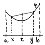 In fact, this is just a more general way to define a convex function. Normally, $φ: [a,b] → ℝ$ is called convex if for every $x, y ∈ [a,b]$, $x < y$, and $0 ≤ λ ≤ 1$, $(1-λ)φ(a)+λφ(b)$ $≥$ $φ((1-λ)a+λb)$. In the language of pictures: all line segments connecting $x$ and $y$, $a ≤ x < y ≤ b$ lie above the graph of the function.
However there is also another way to look at the definition. $(1-λ)a + λb$ is a weighted average of $a$ and $b$, and $(1-λ)φ(a)+λφ(b)$ is a weighted average of $φ(a)$ and $φ(b)$ with the same weights. In other words, $φ$ is convex if and only if for any random variable $X$ such that $\P(X=a) = (1-λ)$, $\P(X=b) = λ$ we have $\E[φ(X)] ≥ φ(\E[X])$, that is, a weighted average of of values of $φ$ is greater (or equal to) the corresponding average of arguments.
This can be further generalized to $X$ taking any finite number of points between $a$ and $b$ by a simple induction, so another way to state the definition of convexity is that for $X$ being a random variable with a finite number of values in $[a,b]$, $\E[φ(X)] ≥ φ(\E[X])$. Since the points can be as “dense” as we want, it is not surprising that it holds for $X$ having any distribution, not necessarily a discrete one.